May 31, 2016

Tao Ren @ Queens College

Problem

Our project is Image Classification and the problem we have for this project is that Machines does not recognize things in the picture. For example, if you give mechine a picture and inside the picture is a dog, how can machines know there is a dog in the picture?  

Goal

The goal for our project is that Feed 50,000 images to training set and use 10,000 to test. And use three different methods to test the accuracy.

DataSet

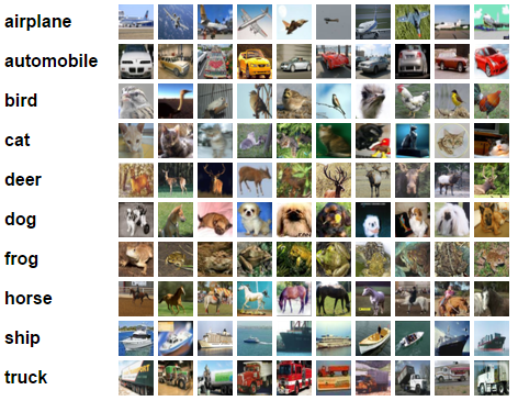
        The DataSet we use is CIFAR-10. CIFAR-10 is a subset of the 80 million tiny images dataset and consists of 60,000 32 * 32 color images containing one of 10 object classes, with 6000 images per class.

Figure 1: The catalog of CIFAR-10, images are from http://www.cs.toronto.edu/~kriz/cifar.html website.

Fractional Max-Pooling with CNN

Overview

Convolutional networks almost always incorporate some form of spatial pooling, and very often it is    max-pooling with  = 2. Max-pooling act on the hidden layers of the network, reducing their size by an integer multiplicative factor . The amazing by-product of discarding 75% of

your data is that you build into the network a degree of invariance with respect to translations and elastic distortions. However, if you simply alternate convolutional layers with max-pooling layers, performance is limited due to the rapid reduction in spatial size, and the disjoint nature

of the pooling regions. A fractional version of max-pooling where  is allowed to take non-integer values. Our version of max-pooling is stochastic as there are lots of different ways of constructing suitable pooling regions.

Convolutional Neural Networks Architecture

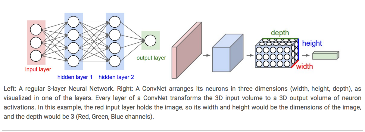
Compared to regular Neural Network, Convolutional Neural Networks take advantage of the fact that the input consists of images and they constrain the architecture in a more sensible way. In particular, unlike a regular Neural Network, the layers of a ConvNet have neurons arranged in 3 dimensions: width, height, depth. (Note that the word depth here refers to the third dimension of an activation volume, not to the depth of a full Neural Network, which can refer to the total number of layers in a network.) The input images in CIFAR-10 are an input volume of activations, and the volume has dimensions 32x32x3 (width, height, depth respectively). As we will soon see, the neurons in a layer will only be connected to a small region of the layer before it, instead of all of the neurons in a fully-connected manner. Moreover, the final output layer would for CIFAR-10 have dimensions 1x1x10, because by the end of the ConvNet architecture we will reduce the full image into a single vector of class scores, arranged along the depth dimension. Here is a visualization:

Layers used to build ConvNets

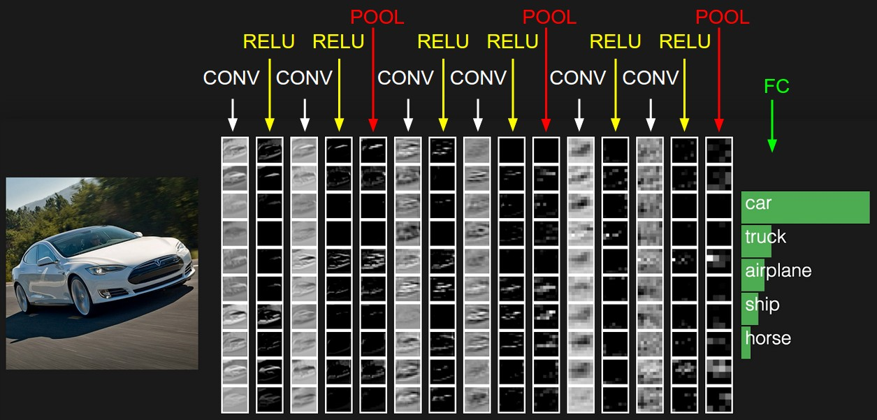
As we described above, a simple ConvNet is a sequence of layers, and every layer of a ConvNet transforms one volume of activations to another through a differentiable function. We use three main types of layers to build ConvNet architectures: Convolutional Layer, Pooling Layer, and Fully-Connected Layer (exactly as seen in regular Neural Networks). We will stack these layers to form a full ConvNet architecture.

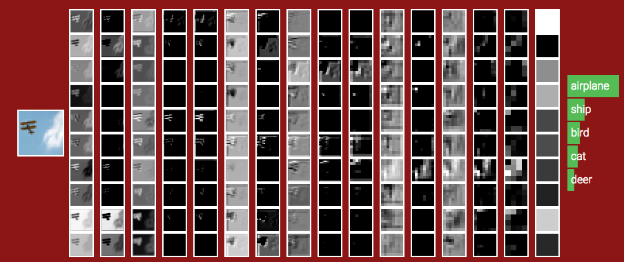
Example Architecture: Overview. We will go into more details below, but a simple ConvNet for CIFAR-10 classification could have the architecture [INPUT - CONV - RELU - POOL - FC]. In more detail:

• INPUT [32x32x3] will hold the raw pixel values of the image, in this case an image of width 32, height 32, and with three color channels R,G,B.
• CONV layer will compute the output of neurons that are connected to local regions in the input, each computing a dot product between their weights and a small region they are connected to in the input volume. This may result in volume such as [32x32x12] if we decided to use 12 filters.
• RELU layer will apply an elementwise activation function, such as the max(0,x) thresholding at zero. This leaves the size of the volume unchanged ([32x32x12]).
• POOL layer will perform a downsampling operation along the spatial dimensions (width, height), resulting in volume such as [16x16x12].
• FC (i.e. fully-connected) layer will compute the class scores, resulting in volume of size [1x1x10], where each of the 10 numbers correspond to a class score, such as among the 10 categories of CIFAR-10. As with ordinary Neural Networks and as the name implies, each neuron in this layer will be connected to all the numbers in the previous volume.

In this way, ConvNets transform the original image layer by layer from the original pixel values to the final class scores. Note that some layers contain parameters and other don’t. In particular, the CONV/FC layers perform transformations that are a function of not only the activations in the input volume, but also of the parameters (the weights and biases of the neurons). On the other hand, the RELU/POOL layers will implement a fixed function. The parameters in the CONV/FC layers will be trained with gradient descent so that the class scores that the ConvNet computes are consistent with the labels in the training set for each image.

Convolutional Layer

The Conv layer is the core building block of a Convolutional Network that does most of the computational heavy lifting.

Overview. The CONV layer’s parameters consist of a set of learnable filters. Every filter is small spatially (along width and height), but extends through the full depth of the input volume. For example, a typical filter on a first layer of a ConvNet might have size 5x5x3 (i.e. 5 pixels width and height, and 3 because images have depth 3, the color channels). During the forward pass, we slide (more precisely, convolve) each filter across the width and height of the input volume and compute dot products between the entries of the filter and the input at any position. As we slide the filter over the width and height of the input volume we will produce a 2-dimensional activation map that gives the responses of that filter at every spatial position. Intuitively, the network will learn filters that activate when they see some type of visual feature such as an edge of some orientation or a blotch of some color on the first layer, or eventually entire honeycomb or wheel-like patterns on higher layers of the network. Now, we will have an entire set of filters in each CONV layer (e.g. 12 filters), and each of them will produce a separate 2-dimensional activation map. We will stack these activation maps along the depth dimension and produce the output volume.

Local Connectivity. When dealing with high-dimensional inputs such as images, as we saw above it is impractical to connect neurons to all neurons in the previous volume. Instead, we will connect each neuron to only a local region of the input volume. The spatial extent of this connectivity is a hyperparameter called the receptive field of the neuron (equivalently this is the filter size). The extent of the connectivity along the depth axis is always equal to the depth of the input volume. It is important to emphasize again this asymmetry in how we treat the spatial dimensions (width and height) and the depth dimension: The connections are local in space (along width and height), but always full along the entire depth of the input volume.

Spatial arrangement. We have explained the connectivity of each neuron in the Conv Layer to the input volume, but we haven’t yet discussed how many neurons there are in the output volume or how they are arranged. Three hyperparameters control the size of the output volume: the depth, stride and zero-padding.

1. First, the depth of the output volume is a hyperparameter: it corresponds to the number of filters we would like to use, each learning to look for something different in the input. For example, if the first Convolutional Layer takes as input the raw image, then different neurons along the depth dimension may activate in presence of various oriented edged, or blobs of color. We will refer to a set of neurons that are all looking at the same region of the input as a depth column (some people also prefer the term fibre).
2. Second, we must specify the stride with which we slide the filter. When the stride is 1 then we move the filters one pixel at a time. When the stride is 2 (or uncommonly 3 or more, though this is rare in practice) then the filters jump 2 pixels at a time as we slide them around. This will produce smaller output volumes spatially.
3. As we will soon see, sometimes it will be convenient to pad the input volume with zeros around the border. The size of this zero-padding is a hyperparameter. The nice feature of zero padding is that it will allow us to control the spatial size of the output volumes (most commonly as we’ll see soon we will use it to exactly preserve the spatial size of the input volume so the input and output width and height are the same).

We can compute the spatial size of the output volume as a function of the input volume size (W), the receptive field size of the Conv Layer neurons (F), the stride with which they are applied (SS), and the amount of zero padding used (P) on the border. You can convince yourself that the correct formula for calculating how many neurons “fit” is given by (W−F+2P)/S+1(W−F+2P)/S+1. For example for a 7x7 input and a 3x3 filter with stride 1 and pad 0 we would get a 5x5 output. With stride 2 we would get a 3x3 output.

Implementation as Matrix Multiplication. Note that the convolution operation essentially performs dot products between the filters and local regions of the input. A common implementation pattern of the CONV layer is to take advantage of this fact and formulate the forward pass of a convolutional layer as one big matrix multiply as follows:

1. The local regions in the input image are stretched out into columns in an operation commonly called im2col. For example, if the input is [227x227x3] and it is to be convolved with 11x11x3 filters at stride 4, then we would take [11x11x3] blocks of pixels in the input and stretch each block into a column vector of size 11*11*3 = 363. Iterating this process in the input at stride of 4 gives (227-11)/4+1 = 55 locations along both width and height, leading to an output matrix X_col of im2col of size [363 x 3025], where every column is a stretched out receptive field and there are 55*55 = 3025 of them in total. Note that since the receptive fields overlap, every number in the input volume may be duplicated in multiple distinct columns.
2. The weights of the CONV layer are similarly stretched out into rows. For example, if there are 96 filters of size [11x11x3] this would give a matrix W_row of size [96 x 363].
3. The result of a convolution is now equivalent to performing one large matrix multiply np.dot(W_row, X_col), which evaluates the dot product between every filter and every receptive field location. In our example, the output of this operation would be [96 x 3025], giving the output of the dot product of each filter at each location.
4. The result must finally be reshaped back to its proper output dimension [55x55x96].

This approach has the downside that it can use a lot of memory, since some values in the input volume are replicated multiple times in X_col. However, the benefit is that there are many very efficient implementations of Matrix Multiplication that we can take advantage of.

Backpropagation. The backward pass for a convolution operation (for both the data and the weights) is also a convolution (but with spatially-flipped filters).

Network-in-Network Layer

An NiN layer is a convolutional layer where the filters have spatial size just 1 x 1. They can be thought of as single layer networks that increase the learning power of a convolutional layer without changing the spatial structure. We placed NiN layers after each max-pooling layer and the final convolutional layer.

Activation function

Leaky ReLU. Leaky ReLUs are one attempt to fix the “dying ReLU” problem. Instead of the function being zero when x < 0, a leaky ReLU will instead have a small negative slope (of 0.33). That is, the function computes f(x)=𝟙(x<0)(αx)+𝟙(x>=0)(x) where α is ⅓.

Softmax classifier

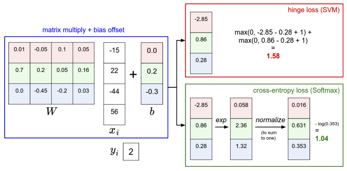
It turns out that the SVM is one of two commonly seen classifiers. The other popular choice is the Softmax classifier, which has a different loss function. If you’ve heard of the binary Logistic Regression classifier before, the Softmax classifier is its generalization to multiple classes. Unlike the SVM which treats the outputs f(xi,W) as (uncalibrated and possibly difficult to interpret) scores for each class, the Softmax classifier gives a slightly more intuitive output (normalized class probabilities) and also has a probabilistic interpretation that we will describe shortly. In the Softmax classifier, the function mapping f(xi;W)=Wxi stays unchanged, but we now interpret these scores as the unnormalized log probabilities for each class and replace the hinge loss with a cross-entropy loss that has the form:

where we are using the notation fj to mean the j-th element of the vector of class scores f. As before, the full loss for the dataset is the mean of Li over all training examples together with a regularization term R(W). The function fj(z)=ezj/∑kezk is called the softmax function: It takes a vector of arbitrary real-valued scores (in z) and squashes it to a vector of values between zero and one that sum to one. The full cross-entropy loss that involves the softmax function might look scary if you’re seeing it for the first time but it is relatively easy to motivate.

Information theory view. The cross-entropy between a “true” distribution p and an estimated distribution qq is defined as:

H(p,q)=−∑xp(x)log⁡q(x)

The Softmax classifier is hence minimizing the cross-entropy between the estimated class probabilities ( q=efyi/∑jefj as seen above) and the “true” distribution, which in this interpretation is the distribution where all probability mass is on the correct class (i.e. p=[0,…1,…,0] contains a single 1 at the yi-th position.).

We can use the cross-entropy loss to train the convolutional neural network.

Spatial sparsity for convolutional networks

Imagine putting an all-zero array into the input layer of a CNN. As you evaluate the network in the forward direction, the translational invariance of the input is propagated to each of the hidden layers in turn. We can therefore think of each hidden variable as having a ground state corresponding to receiving no meaningful input; the ground state is generally non-zero because of bias terms. When the input array is sparse, you only have to calculate the values of the hidden variables where they differ from their ground state. Figure S1 shows how the active spatial locations change through the layers.

Figure S1: The active spatial locations (black) when a circle with diameter 32 is placed in the center of a 94 × 94 input layer and fed forward. Sparsity is most important in the early stages where most of the spatial locations are in their ground state (gray).

Essentially, we want to memoize the convolutional and pooling operations. Memoizing can be done using a hash table, but that would be inefficient here as for each operation there is only one input, corresponding to regions in the ground state, that we expect to see repeatedly.

Instead, to forward propagate the network we calculate two matrices for each layer of the network:

• A feature matrix which is a list of row vectors, one for the ground state, and one for each active spatial location in the layer; the width of the matrix is the number of features per spatial location.
• A pointer matrix with size equal to the spatial size of the convolutional layer. For each spatial location in the convolutional layer, we store the number of the corresponding row in the feature matrix.

This representation is very loosely biologically inspired. The human visual cortex separates into two streams of information: the dorsal (where) and ventral (what) streams. Similar data structures can be used in reverse order for backpropagation.

For a regular convolutional network, the convolutional and pooling operations within a layer can be performed in parallel on a GPU (or even spread over multiple GPUs). Exactly the same holds here; there is simply less work to do as we know the inactive output spatial locations are all the same.

Dropout

Model combination nearly always improves the performance of machine learning methods. With large neural networks, however, the obvious idea of averaging the outputs of many separately trained nets is prohibitively expensive. Combining several models is most helpful when the individual models are different from each other and in order to make neural net models different, they should either have different architectures or be trained on different data. Training many different architectures is hard because finding optimal hyperparameters for each architecture is a daunting task and training each large network requires a lot of computation. Moreover, large networks normally require large amounts of training data and there may not be enough data available to train different networks on different subsets of the data. Even if one was able to train many different large networks, using them all at test time is infeasible in applications where it is important to respond quickly.

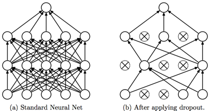
Figure D1

Dropout is a technique that addresses both these issues. It prevents overfitting and provides a way of approximately combining exponentially many different neural network architectures efficiently. The term “dropout” refers to dropping out units (hidden and visible) in a neural network. By dropping a unit out, we mean temporarily removing it from the network, along with all its incoming and outgoing connections, as shown in Figure D1. The choice of which units to drop is random. In the simplest case, each unit is retained with a fixed probability p independent of other units, where p can be chosen using a validation set or can simply be set at 0.5, which seems to be close to optimal for a wide range of networks and tasks. For the input units, however, the optimal probability of retention is usually closer to 1 than to 0.5.

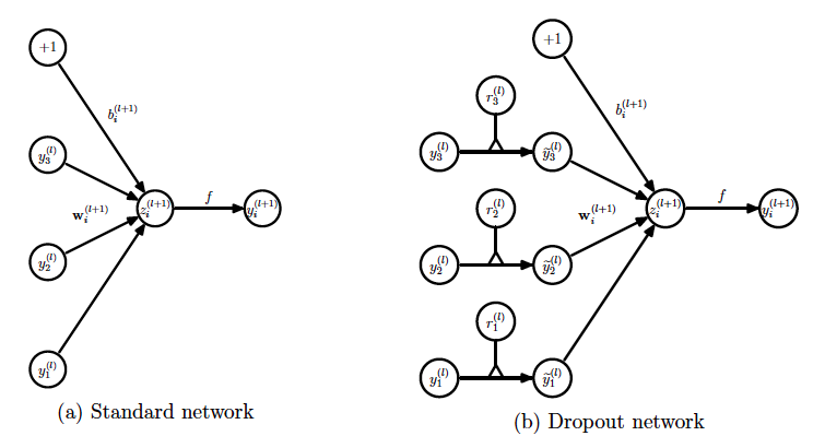
Figure D2

Applying dropout to a neural network amounts to sampling a “thinned” network from it. The thinned network consists of all the units that survived dropout (Figure D1.b). A neural net with n units, can be seen as a collection of 2n possible thinned neural networks. These networks all share weights so that the total number of parameters is still O(n2), or less. For each presentation of each training case, a new thinned network is sampled and trained. So training a neural network with dropout can be seen as training a collection of 2n thinned networks with extensive weight sharing, where each thinned network gets trained very rarely, if at all.

At test time, it is not feasible to explicitly average the predictions from exponentially many thinned models. However, a very simple approximate averaging method works well in practice. The idea is to use a single neural net at test time without dropout. The weights of this network are scaled-down versions of the trained weights. If a unit is retained with probability p during training, the outgoing weights of that unit are multiplied by p at test time as shown in Figure D2. This ensures that for any hidden unit the expected output (under the distribution used to drop units at training time) is the same as the actual output at test time. By doing this scaling, 2n networks with shared weights can be combined into a single neural network to be used at test time. We found that training a network with dropout and using this approximate averaging method at test time leads to significantly lower generalization error on a wide variety of classification problems compared to training with other regularization methods.

Consider a neural network with L hidden layers. Let l{1,...,L} index the hidden layers of the network. Let z(l) denote the vector of inputs into layer l, y(l) denote the vector of outputs from layer l (y(0) = x is the input). W(l) and b(l) are the weights and biases at layer l. The feed-forward operation of a standard neural network can be described as (for l{1,...,L} and any hidden unit i)

zi(l+1)  = wi(l+1) yl + bi(l+1) ,

yi(l+1)  = f(zi(l+1) ) ,

where f is the activation function, here is Leaky ReLU:

With dropout, the feed-forward operation becomes

rj(l)      ~ Bernoulli(p),

(l)    = r(l) * y(l),

zi(l+1)  = wi(l+1)(l) + bi(l+1) ,

yi(l+1)  = f(zi(l+1) ) ,

Here * denotes an element-wise product. For any layer l, r(l) is a vector of independent Bernoulli random variables each of which has probability p of being 1. This vector is sampled and multiplied element-wise with the outputs of that layer, y(l), to create the thinned outputs (l). The thinned outputs are then used as input to the next layer. This process is applied at each layer. This amounts to sampling a sub-network from a larger network. For learning, the derivatives of the loss function are backpropagated through the sub-network. At test time, the weights are scaled as Wtest(l)= pW(l). The resulting neural network is used without dropout.

Fractional max-pooling (FMP)

The idea of FMP is to reduce the spatial size of the image by a factor of   with 1 < α  < 2 . Like stochastic pooling, FMP introduces a degree of randomness to the pooling process. However, unlike stochastic-pooling, the randomness is related to the choice of pooling regions, not the way pooling is performed inside each of the pooling regions. Briefly, there are three choices that affect the way FMP is implemented:

• The pooling fraction which determines the ratio between the spatial sizes of the input and the output of the pooling layer. Regular 2 x 2  max-pooling corresponds to the special case α = 2 .
• The pooling regions can either be chosen in a random or a pseudorandom fashion. There seems to be a trade off between the use of randomness in FMP and the use of dropout and/or training data augmentation. Random-FMP seems to work better on its own; however, when combined with ‘too much’ dropout or training data augmentation, underfitting can occur.
• The pooling regions can be either disjoint or overlapping. Disjoint regions are easier to picture, but we find that overlapping regions work better.

Each convolutional filter of a CNN produces a matrix of hidden variables. The size of this matrix is often reduced using some form of pooling. Max-pooling is a procedure that takes an Nin × Nin input matrix and returns a smaller output matrix, say Nout × Nout. This is achieved by dividing the Nin × Nin square into Nout2 pooling regions (Pi,j ):

Pi,j ⊂ {1, 2, . . . , Nin}2 for each (i, j) ∈ {1, . . . , Nout}2

and then setting

If we take Nin/Nout ≈ then the rate of decay of the spatial size of interesting features is n times slower. For clarity we will now focus on the case Nin/Nout ∈ (1, 2) as we are primarily interested in accuracy; if speed is an overbearing concern then FMP could be applied with Nin/Nout ∈ (2, 3).

Given a particular pair of values (Nin, Nout) we need a way to choose pooling regions (Pi,j ). We will consider two type of arrangements, overlapping squares and disjoint collections of rectangles. In Figure F1 we show a number of different ways of dividing up a 36 × 36 square grid into disjoint rectangles. Pictures two, three and six in Figure F1 can also be used to define an arrangement of overlapping 2 × 2 squares: take the top left hand corner of each rectangle in the picture to be the top left hand corner of one of the squares.

Figure F1

To give a formal description of how to generate pooling regions, let (ai)i=0Nout and (bi)i=0Nout be two increasing sequence of integers starting at 1, ending with Nin, and with increments all equal to one or two (i.e. ai+1 − ai ∈ {1, 2}). The regions can then be defined by either

P = [ai−1, ai − 1] × [bj−1, bj − 1] or Pi,j = [ai−1, ai] × [bj−1, bj].

We call the two cases disjoint and overlapping, respectively. We have tried two different approaches for generating the integer sequence: using random sequences of numbers and also using pseudorandom sequences.

We will say that the sequences are random if the increments are obtained by taking a random permutation of an appropriate number of ones and twos. We will say that the sequences are pseudorandom if they take the form

ai = ceiling(α(i + u)), α ∈ (1, 2), with some u ∈ (0, 1).

Below are some patterns of increments corresponding to the case Nin = 25, Nout = 18. The increments on the left were generated ‘randomly’, and the increments on the right come from pseudorandom sequences:

211112112211112122        112112121121211212

111222121121112121        212112121121121211

121122112111211212        211211212112121121

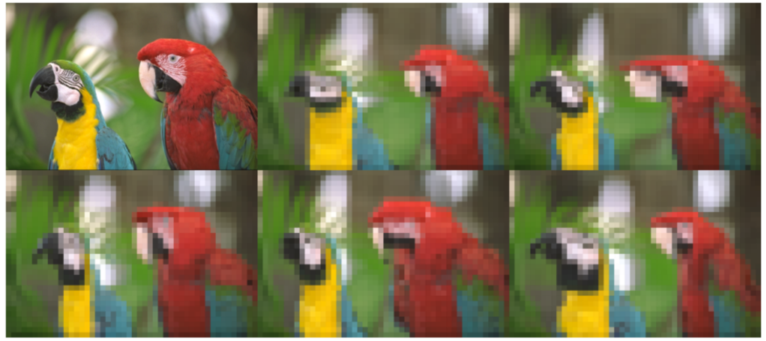
Although both types of sequences are irregular, the pseudorandom sequences generate much more stable pooling regions than the random ones. To show the effect of randomizing the pooling regions, see Figure F2. We have taken a picture, and we have iteratively used disjoint random pooling regions to reduce the size of the image (taking averages in each pooling region). The result is that the scaled down images show elastic distortion. In contrast, if we use pseudorandom pooling regions, the resulting image is simply a faithfully scaled down version of the original.

Figure F2: Top left, ‘Kodak True Color’ parrots at a resolution of 384 × 256. The other five images are one-eighth of the resolution as a result of 6 layers of average pooling using disjoint random FMP-pooling regions.

RNG

Random number generator, which is used in this project for dropout and fmp, has some functions:

• uniform(a, b): Generates uniformly distributed integer random number from [a,b)
• normal: Generates random numbers according to the Normal (or Gaussian) random number distribution:
• bernoulli: Produces random boolean values, according to the discrete probability function:
• NchooseM: Generates the n choose m row randomization matrix/vector. If we want to do dropout, e.g. N input features needs to drop to M output features, NchooseM can generate M random unique index, which we can keep that related M features, and the remain features are dropped.
• permutation: Generates a shuffled number sequence: {0,1,...,n-1}. If we want to generate a random pooling regions, we can create an integer array filled with appropriate number of ones and twos, using permutation to generate a shuffled index sequence, accordingly, a shuffled ones and twos.

Model

Using a random overlapping pooling FMP network, there is a dropout layer between every C2 and FMP layer.

C2: filterSize = 2

  std::cout << "Convolution "

            << filterSize <<"^" <<dimension<< "x"<< nFeaturesIn

            << "->" << nFeaturesOut;

F=2, S=1 W1=94, D1=3, P=0

W2 = 93, D2=12==>32

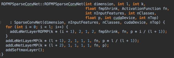
ROFMPSparseConvNet::ROFMPSparseConvNet

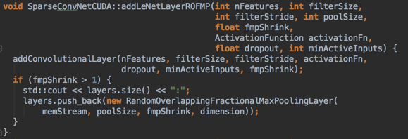
addLeNetLayerROFMP() (SparseConvNetCUDA.cu)

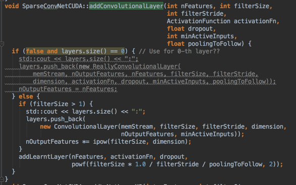
→ addConvolutionalLayer()

push( ConvolutionalLayer )

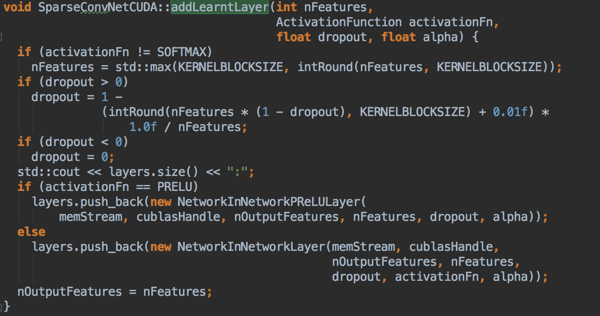
        → addLearntLayer()

                push( NetworkInNetworkLayer )

→push( RandomOverlappingFractionalMaxPoolingLayer )

addLeNetLayerMP()

→ addConvolutionalLayer()

        → push( MaxPoolingLayer )

addLeNetLayerMP()

addSoftmaxLayer()

→ addLearntLayer()

Dimension: 2

l: 12 (i = 0; i < l; i+)

k: 32

fmpShrik:

ActivationFunction: VLEAKRELU

Input Features: 3

Input Class: 10

dropout - p: 0.1

ConvolutionalLayer:

Features: k * (i + 1)

filterSize: 2

filterStride: 1

poolSize: 2

fmpShrink:

dropout: p * i / (l + 1)

LearntLayer:

Features, activationFn, dropout, (filterSize/filterStride/poolingToFollow)^2

poolingToFollow==fmpShrink

NetworkInNetworkLayer

ROFMP:

poolsize, fmpShrink, dimension

Layer sizes of the network:

[output]-1-(C1)-1-(C2)-2-(ROFMP)-3-(C2)-4-(ROFMP)-5-(C2)-6-(ROFMP)-8-(C2)-9-(ROFMP)-11-(C2)-12-(ROFMP)-15-(C2)-16-(ROFMP)-20-(C2)-21-(ROFMP)-26-(C2)-27-(ROFMP)-34-(C2)-35-(ROFMP)-44-(C2)-45-(ROFMP)-57-(C2)-58-(ROFMP)-73-(C2)-74-(ROFMP)-93-(C2)-94-[Input]

Using 50,000 pictures as training set, other remaining 10,000 pictures as test set.

CNN Model to be trained:

(32nC2 - ROFMP)12 - C2 -C1 - output.

ROFMP: Pseudorandom Overlapping Fractional Maxing-out Pooling

Extra Dataset into Spatially Sparse Dataset

The SparseConvNet project that we are using read dataset directly from bin format into Spatially Sparse Dataset which combine 3 separated channel data into one pixel.

According to  the CNN Model: (32nC2 - ROFMP)12 - C2 -C1 - output, we can calculate that the training input data’s spatial size should be 94x94. The actual input picture’s size is 32x32, which will place at the center of a 94x94 sparse grid after the augmentation(see below).

Training Data Augmentation

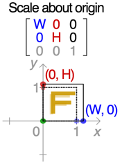
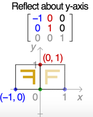
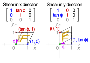
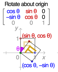
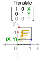
We extended the training set using affine transformations: a randomized mix of scaling, reflections, shearing, rotations, and translation operations. We also added random shifts to the pictures in RGB colorspace.

W-scale: 0.8~1.2;

H-scale: 0.8~1.2;

Horizontal flip: 50%;

X-shear: 33% (: -0.2~0.2)

Y-Shear: 33% (: -0.2~0.2)

Rotation: 33% (: -0.2~0.2)

X-translate (offset): -16 ~ 16 pixels

Y-translate (offset): -16 ~ 16 pixels

Color Distortion:

Model averaging

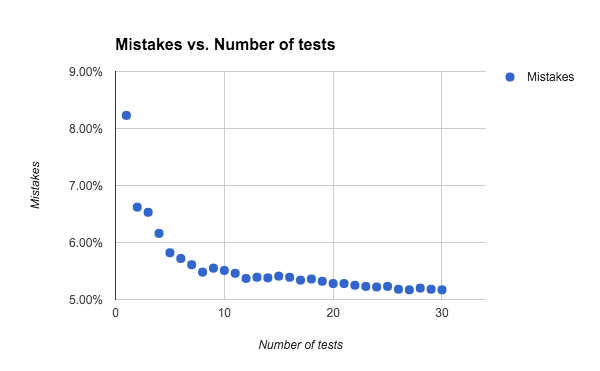
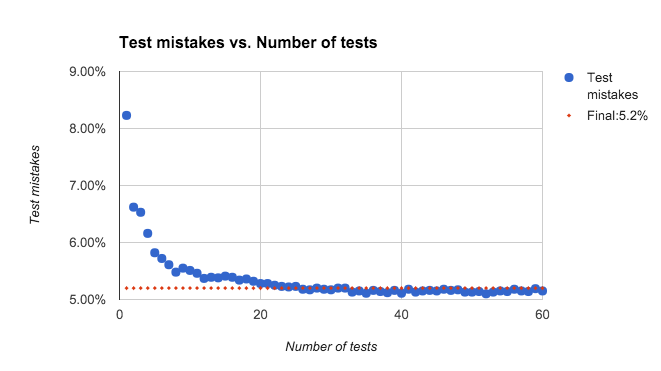
Each time we apply an FMP network, either for training or testing purposes, we use different random or pseudorandom sequences to generate the pooling regions. An FMP network can therefore be thought of as an ensemble of similar networks, with each different pooling-region configuration defining a different member of the ensemble. This is similar to dropout; the different values the dropout mask can take define an ensemble of related networks. As with dropout, model averaging for FMP networks can help improve performance. If you classify the same test image a number of times, you may get a number of different predictions. Using majority voting after classifying each test image a number of times can substantially improve accuracy; see below.

Implementation

We are using an open source project in: https://github.com/btgraham/SparseConvNet

We are using a Mac Pro to run the program, with configuration:

• Mac OS 10.11
• Intel Core i7 2.30GHz CPU
• 16 GB 1600 MHz DDR3 RAM
• 500GB SSD
• NVIDIA GeForce GT 750M 2048 MB

Because it’s a c++ project, need to build using cuda in Ubuntu, we have to change the code a little bit to let the compiler(nvcc) work. Besides, the network training needs around 1.5G memory space, while the GPU just has 750MB free space, we have to change the memory allocation from GPU to main memory, causing the performance drops to 500 seconds per epoch.

It takes 213382 seconds for training 410 epochs to the network, which is almost 60 hours.

Result

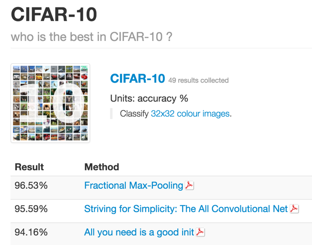
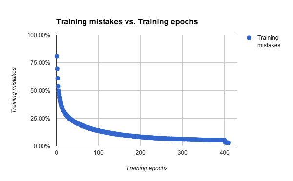
The original project achieves 96.53% accuracy, and the project we use achieves 94.8% accuracy after 410 epochs training, the test error of the network is around 5.2%. The network’s training mistake drop suddenly from 5.4% to 2.99% after 400 epochs, seems it has over-fitted and we stop the training.

Conclusion

We use three different methods to test the accuracy. The first method is Convolutional Neural Networks By Caffe, it is comprised of many convolutional layers. The Accuracy of this method is 78%. Although it is not very high accuracy, the executed time is impressive. The second method is Histogram of Oriented Gradients and linear support vector Machine. HOG features can be described as taking a nonlinear function of the edge orientations in an image and pooling them into small spatial regions to remove sensitivity to exact localisation of the edges. This type of representation has proven particularly successful at being tolerant to non-rigid changes in object geometry whilst maintaining high selectivity.The last method is Fractional max-Polling with CNN, it trained convolutional networks with fractional max-pooling on a number of popular datasets. Although it has high accuracy, the execution time is extremely slow.

Reference

• CIFAR-10, https://www.kaggle.com/c/cifar-10 
• CNN with fractional max-pooling: http://arxiv.org/pdf/1412.6071v4.pdf
• CNN: http://cs231n.github.io/convolutional-networks/
• Spatially-sparse convolutional neural networks:
  http://arxiv.org/pdf/1409.6070v1.pdf;
  https://github.com/btgraham/SparseConvNet;
  https://github.com/btgraham/SparseConvNet/wiki/Installation
  
• Dropout: http://jmlr.org/papers/volume15/srivastava14a/srivastava14a.pdf
• CUDA: https://github.com/BVLC/caffe/wiki/Ubuntu-14.04-VirtualBox-VM
• Neural Network: http://cs231n.github.io/neural-networks-1/
• Affine Transformation: https://en.wikipedia.org/wiki/Transformation_matrix